Worked Examples: Hyperbolic, Parabolic, and Elliptic Equations

Hyperbolic equation example

The typical example of a hyperbolic equation is the wave equation:

$\frac{\partial^2 u}{\partial t^2} - a^2\frac{\partial^2 u}{\partial x^2} = 0$

An exact solution can be determined as:

$u(x,t) = a \cdot \sin(\pi x) \cdot \cos(\pi t)$

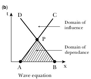
Using the characteristic-curve coefficients from the previous lesson, this equation yields two real characteristics. The set of characteristic equations are two straight lines (because $a$ is a constant), which show that a disturbance:

$\begin{cases} \dfrac{\mathrm{d}x}{\mathrm{d}t} = a \\[4pt] \dfrac{\mathrm{d}x}{\mathrm{d}t} = -a \end{cases}$

taking place at point P influences the solution domain after P (region CPD). The solution at point P is influenced by disturbances in the domain before point P (region APB). Depending on the position of P in the computational domain, initial conditions may be sufficient to determine the solution at point P uniquely.

Parabolic equation example

The typical example of a parabolic equation is the diffusion of a pollutant in a water body. The diffusion equation in one dimension of space is:

$\frac{\partial u}{\partial t} = D\frac{\partial^2 u}{\partial x^2}$

where $D$ is the diffusion coefficient. The analytical solution is:

$u(x,t) = \sin(\pi x) \cdot \exp(-\pi^2 t)$

The exponential part of the solution represents the time decay. When other types of boundary and initial conditions are given, the solution has to be computed either through integration or through numerical approximation. In the case of parabolic equations, characteristics are not so important because they are equal ($C_1 = C_2$), and they show that the solution at point P of the computational space can influence any point in the computational domain. Any combination of Dirichlet, Neumann, or Robin boundary conditions is appropriate to use.

Elliptic equation example

Elliptic equations are time-independent and therefore only valid in the case of steady flows. A typical example of an elliptic equation is the Laplace equation:

$\frac{\partial^2 u}{\partial x^2} + \frac{\partial^2 u}{\partial y^2} = 0$

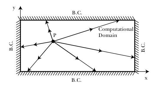
In the case of elliptic PDEs, all boundary conditions should be given. The characteristic lines are of complex (imaginary) nature and cannot be represented in the real domain, hence they are not used. The important characteristic of an elliptic equation is that any disturbance at point P in the computational domain will influence all the points in the computational domain.