Solving ODEs and PDEs

Solution of an ODE

The general form of an ODE is:

$\frac{\mathrm{d}u(t)}{\mathrm{d}t} = f(u, t)$

where $u(t)$ is an unknown function of the variable $t$ (time) and $f$ is an arbitrary function of $u(t)$ and $t$. Ordinary differential equations may have analytical solutions that are easy to obtain if the function $f(u, t)$ is not too complicated. However, even if an analytical solution exists, implementing that solution into a computer programme may be difficult. If, along with the equation, an initial value of the function $u(x, t)$ is given, the problem is called an initial value problem (IVP) and can be solved easily using numerical approximations.

Solution of a PDE

In order to have a solution for a PDE, the problem must be well posed mathematically. This implies that the solution fulfils three conditions:

• the solution exists,
• the solution is unique,
• the solution depends on auxiliary conditions such as boundary conditions.

Fletcher (1998) states that uniqueness of solution is not a problem in general, and if it does not exist it is mainly due to failure to fulfil auxiliary conditions. However, there are physical phenomena for which multiple solutions exist, due to the physical phenomena itself rather than the mathematical position of the problem — such as the transition from laminar to turbulent flow.

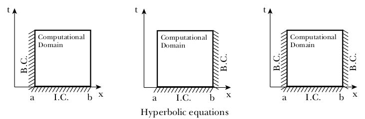
Any PDE can be solved if boundary conditions and initial conditions on the computational domain are known. Typical representations of the computational domain and required boundary conditions for hyperbolic PDEs look like this:

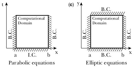
And for parabolic and elliptic PDEs:

Types of boundary conditions

The definition of boundary conditions constitutes the start for determining the solution of any problem inside the computational domain. There are three ways of defining boundary conditions:

• Dirichlet type: when the values of the unknown function $u$ are known at the border of the computational volume.
• Neumann type: when derivatives of the unknown function are known at the border of the computational domain.
• Robin (mixed) type: when a combination of Dirichlet and Neumann conditions are applied at the domain boundary.

Errors

An important issue in finding the solution of a PDE is errors. Hyperbolic types of problems are the most exposed to errors, because in their case conditions at the boundary of the computational domain are the ones introducing errors that will propagate inside the computational domain.