Characteristics and Boundary Conditions for Fluid Flow PDEs

The majority of flow phenomena in hydraulics (hydrodynamics) are governed by a system of two differential equations (as is the case, for example, for free surface flows). A system of two first-order partial differential equations, having two independent variables ($\xi, \eta$) and two unknown functions ($u$ and $v$), is written as:

$a_1\frac{\partial u}{\partial \xi} + b_1\frac{\partial u}{\partial \eta} + c_1\frac{\partial v}{\partial \xi} + d_1\frac{\partial v}{\partial \eta} = f_1$

$a_2\frac{\partial u}{\partial \xi} + b_2\frac{\partial u}{\partial \eta} + c_2\frac{\partial v}{\partial \xi} + d_2\frac{\partial v}{\partial \eta} = f_2$

where $\xi$ and $\eta$ are the independent variables. For water-related problems, $\xi$ corresponds to the $x$-coordinate and $\eta$ to time $t$. The unknown functions are variables that correspond to flow quantities, such as flow velocity or water depth $h$.

Deriving the characteristic curves

Because both $u$ and $v$ are functions of $(\xi, \eta)$, their total derivatives in the $(\xi, \eta)$ plane are:

$\mathrm{d}u = \frac{\partial u}{\partial \xi}\mathrm{d}\xi + \frac{\partial u}{\partial \eta}\mathrm{d}\eta \qquad \mathrm{d}v = \frac{\partial v}{\partial \xi}\mathrm{d}\xi + \frac{\partial v}{\partial \eta}\mathrm{d}\eta$

These derivatives can have different values in different regions of the $(\xi, \eta)$ plane, or may not exist in some regions. The curves splitting the plane into these different regions are called characteristic curves, determined from the condition that the determinant of the system formed from the four equations above is not zero. If the determinant of the system is not zero, the system of equations has a unique solution.

Writing the formed system in matrix format:

$\begin{bmatrix} a_1 & b_1 & c_1 & d_1 \\ a_2 & b_2 & c_2 & d_2 \\ \mathrm{d}\xi & \mathrm{d}\eta & 0 & 0 \\ 0 & 0 & \mathrm{d}\xi & \mathrm{d}\eta \end{bmatrix} \begin{bmatrix} \partial u/\partial \xi \\ \partial u/\partial \eta \\ \partial v/\partial \xi \\ \partial v/\partial \eta \end{bmatrix} = \begin{bmatrix} f_1 \\ f_2 \\ \mathrm{d}u \\ \mathrm{d}v \end{bmatrix}$

The unknowns of the system are the derivatives of $u$ and $v$. These are not determined if the determinant of the system is zero — the value zero of the determinant defines the regions in space beyond which there is no solution for the given equation, because the derivatives do not exist. Setting the determinant to zero:

$\begin{vmatrix} a_1 & b_1 & c_1 & d_1 \\ a_2 & b_2 & c_2 & d_2 \\ \mathrm{d}\xi & \mathrm{d}\eta & 0 & 0 \\ 0 & 0 & \mathrm{d}\xi & \mathrm{d}\eta \end{vmatrix} = 0$

Calculating the determinant and rearranging yields a quadratic in $\mathrm{d}\eta/\mathrm{d}\xi$:

$a\left(\frac{\mathrm{d}\eta}{\mathrm{d}\xi}\right)^2 + b\frac{\mathrm{d}\eta}{\mathrm{d}\xi} + c = 0$

with coefficients $a = (a_1c_2 - a_2c_1)$, $b = (-a_1d_2 + a_2d_1 - b_1c_2 + b_2c_1)$, $c = (b_1d_2 - b_2d_1)$. This has two solutions, real or imaginary depending on the discriminant, given by the quadratic formula:

$\frac{\mathrm{d}\eta}{\mathrm{d}\xi} = \frac{-b \pm \sqrt{b^2 - 4ac}}{2a}$

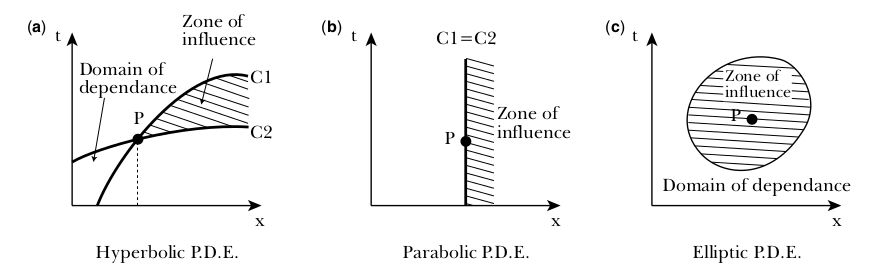
The solutions represent curves in the $(\xi, \eta)$ plane, called characteristic curves ($C_1$ and $C_2$), and determine the number of required boundary conditions needed for a unique solution. The discriminant here is similar to the one defining the types of PDEs, so depending on its value the problem can be of 3 types:

• Hyperbolic — with two real characteristics.
• Parabolic — with one characteristic ($C_1 = C_2$).
• Elliptic — with two imaginary characteristics.

Domain of influence and domain of dependence

Domain of influence: This is the region that can be affected by what happens at a given point or region. For water-related problems, imagine dropping a stone in a pond: the ripples spread out from the point of impact, and the area these ripples can reach is the domain of influence — it represents all points that can be affected by the initial disturbance.

Domain of dependence: This is the region that determines the solution at a specific point. Using the pond analogy: to know the water height at a specific point after 1 second, you need to know the initial conditions in a certain region around that point — this region is the domain of dependence.